Marginal revenue productivity (MRPL) is a theory of wages where workers are paid the value of their marginal revenue product to the firm.
The MRP theory outlined below is based on the assumption of a perfectly competitive labour market and the theory rests on a number of key assumptions that realistically are unlikely to exist in the real world. Most labour markets are imperfect, one of the reasons for earnings differentials between occupations which we explore a little later on.
Workers are homogeneous in terms of their ability and productivity
Firms have no buying power when demanding workers (i.e. they have no monopsony power)
There are no trade unions (the possible impact on unions on wage determination is considered later)
The productivity of each worker can be clearly and objectively measured and the value of output can be calculated
The industry supply of labour is assumed to be perfectly elastic. Workers are occupationally and geographically mobile and can be hired at a constant wage rate
Marginal Revenue Product (MRPL) measures the change in total output revenue for a firm as a result of selling the extra output produced by additional workers employed. A straightforward way of calculating the marginal revenue product of labour is as follows:
MRPL = Marginal Physical Product x Price of Output per unit
Therefore the MRP curve represents the firm’s demand for labour curve and the profit maximising condition is where:
MRPL = MCL (Marginal Cost of Labour) where the revenue generating by employing an additional worker (MRPL) = the cost of employing an additional worker (MCL).
Mind Map below adapted from Susan Grant’s book CIE A Level Revision Guide
Use elearneconomics for immediate personalised feedback on Marginal Revenue Productof Labour with tasks designed for true student-centred learning and understanding that improves students results and grades.
Below is a very good video from CNBC that covers the main causes of recessions – overheated economy, asset bubbles and black swan events. Good analysis of soft and hard landings as well as the wage price spiral effect.
“History teaches us that recessions are inevitable,” said David Wessel, a senior fellow in economic studies at The Brookings Institution. “I think there are things we can do with a policy that makes recessions less likely or when they occur, less severe. We’ve learned a lot, but we haven’t learned enough to say that we’re never going to have another recession.” As the nation’s authority on monetary policies, the Federal Reserve plays a critical role in managing recessions. The Fed is currently attempting to avoid a recession by engineering what’s known as a “soft landing,” in which incremental interest rate hikes are used to curb inflation without pushing the economy into recession.
There has much debate around the benefits of the four-day working week for both employees and employers. Research which was co-ordinated by a not-for-profit organisation, 4 Day Week Global, with employers in Ireland, the United States, Australia and New Zealand taking part. The UK had the biggest single-country trial in 2022 (Covid-19) which involved 73 companies and 3,300 employees. The Statista graphic below shows the results of the study which mainly focuses on productivity.
Why do economies put significant emphasis on boosting productivity?
Higher wages – with greater output per unit of input firms can offset the effect of wage increase on profits.
Lower prices – with productivity increasing businesses can pass on lower prices to consumers, although whether this actually happens is another story.
Higher profits – with productivity going up businesses can increase in their profits which means more money can be reinvested into the firm
Higher potential growth – higher productivity is the main driver of living standards and shifting the production possibility curve (PPC) outwards.
Other data from the research
Declining levels of stress, burnout and general fatigue
Better physical and mental health and work-life balance
Although some still worked on their day off, most felt more productive
Greater levels of exercise and sleep
Male workers spent more time looking after their children – up by 27%.
One less day at work meant less commuting time and therefore less environmental impact
Juliet Schor, an economist and sociologist at Boston College and lead researcher at 4 Day Week Global argues that a shorter working week is key to achieving the carbon emissions reductions the world needs. Click here to listen to her interview on the IMF podcast series ‘Women in Economics” Juliet Schor on the Benefits of the 4-day week.
“Although climate benefits are the most challenging thing to measure, we have a lot of research showing that over time, as countries reduce hours of work, their carbon emissions fall. A 10% reduction in hours is associated to an 8.6% fall in carbon footprint” according to a study co-authored by Schor in 2012
For more on the Labour Market view the key notes (accompanied by fully coloured diagrams/models) on elearneconomics that will assist students to understand concepts and terms for external examinations, assignments or topic tests.
The Liverpool v Chelsea Carabao Cup Final was seen as an opportunity for Chelsea’s new owners to get their hands on some silverware. Chelsea must have fancied their chances with the Liverpool side fielding five academy players and missing the likes of Mo Salah, Trent Alexander-Arnold, Joel Matip, Alisson, Curtis Jones, Diogo Jota, Thiago Alcantara, Darwin Núñez and Stefan Bajcetic. As a consequence the value of both teams at the final whistle was very unequal. Chelsea being valued at £521m and Liverpool £163.3m – see image.
However as a manager of a football team one of the most important aspects of the job is motivating your players and developing a winning culture. Jurgen Klopp fostered a sense of unity, commitment, and resilience among his players, which is crucial to their success. Faced with these numerous injuries his ability to inspire players in difficult times was evident in the Carabao Cup Final. Also Klopp’s willingness to experiment with new formations and younger players demonstrated his commitment to improvement and depth in the squad.
Klopp’s emphasis on teamwork and camaraderie can serve as an inspiration and it draws on parallels between his role as a football manager and that of a CEO in which there is a transferability of key leadership attributes.
For more on Labour Economics view the key notes (accompanied by fully coloured diagrams/models) on elearneconomics that will assist students to understand concepts and terms for external examinations, assignments or topic tests.
Tiger Woods was in the news recently with the ending of his relationship with the apparel company ‘Nike’ which was worth $660m over three decades. Has he signed a deal with another company? We will find out what Woods will sport in the Genesis Invitational at Riviera Country Club in February and throughout the rest of 2024.
As with any elite athlete there comes a time when the value of endorsements / sponsorship etc and accumulated past income allows them to achieve greater utility levels without working. This concept refers to the income and substitution effect and the backward bending supply curve of labour. Economic theory assumes that there is a positive relationship between labour supply and the wage rate. So, as the wage rate increases, more people are willing to work. This is represented by the individual’s labour supply curve, which mainly slopes upwards. Beyond a certain point, individuals will take the view that they prefer leisure to work. This point is indicated by the backward-sloping curve from point S’. Before this point, an individual worker is more willing to supply his or her labour as the wage rate increases. It must be stressed that this point depends on the individual’s attitude to work and leisure – point S’ on any individual’s supply curve will vary (see graph above).
Therefore professional athletes who reach a certain level of performance, whether it be in golf, tennis, cycling etc tend not to take part in so many events because of their increase in wealth. Appearance money, endorsements as well as prize money mean the income effect increases as the athlete can, in theory, achieve greater utility levels without performing. This may be more prevalent as the athlete enters the latter stages of his/her career. So with Tiger Woods appearing next at Genesis Invitational at Riviera Country Club in February what company will he be endorsing and how many tournaments will he play in 2024?
Source: The Economics of Sport – Leeds, von Allmen and Matheson (2018)
Sign up to elearneconomics for comprehensive key notes with coloured illustrations, flash cards, written answers and multiple-choice tests on the Supply of Labour that provides for users with different learning styles working at their own pace (anywhere at any time).
One reason for the increasing inequality in society is the stagnant wages for the lower and middle income groups – in the USA the top 0.1% have as much wealth as the bottom 90%. Labour compensation at the very top has increased dramatically since the 1970’s.
1970’s – the top 0.1% took home less than 3% of all income 2010 – the top 0.1% took home more than 10% of all income
In the USA the top CEO’s average compensation has grown since the late 1970’s by over 900% to around $15 million a year. In contrast the lower income groups have gone up by only 10%. However when you look at hedge fund and private equity fund managers the salaries are astounding. In 2014 which was seen as not a great year for the industry 25 fund managers made at least $175 million each, and 3 made more than $1 billion.
Are CEO’s worth every cent?
In theory the demand for labour is determined by their marginal revenue product – that is the value of revenue generating by employing an additional worker. Labour markets are imperfect and a monopsony occurs in the labour market when there is a single or dominant buyer of labour. The buyer therefore is able to determine the price at which is paid for services. The monopsonist will hire workers where:
Marginal Cost of labour (MCL) = Marginal Revenue product of labour (MRPL)
Therefore it will use labour up to level of Eq which is where MCL=MRPL. In order to entice workers to supply this amount of labour, the firm need pay only the wage Wq. (Remember that ACL is the supply of labour). You can see, therefore, that a profit-maximising monopsonist will use less labour, and pay a lower wage, than a firm operating under perfect competition.
So if Goldman Sach’s CEO, Lloyd Blankfein, made $24 million in 2014, that’s because he is worth $24 million to his company. In short, you make what you deserve based on your skills, effort, and productivity, in this fairest of all possible worlds.
However this theory has little to do with how the world actually works. The idea that good CEO’s are entitled to enormous rewards is based on the belief that success or failure of the company depends on one person. According to historian Nancy Koehn, business is a team sport: not only is it impossible to quantify a single leader’s marginal revenue product; it is hard even to describe it clearly. Ultimately a CEO can appoint friends and place them on the compensation committee which recommends the CEO salary. The committee invariably proposes to pay at least as much as the median comparable company, because no board wants to admit that its company has a below-average leader. CEO’s do have key performance indicators (KPI’s) but the CEO can encourage the committee to select metrics that will be easy to satisfy. John Kenneth Galbraith describes CEO pay very succinctly – “The salary of the chief executive of a large corporation is not a market reward for achievement. It is frequently in the nature of a warm personal gesture by the individual to himself.”
Luck plays an important role in CEO’s pay. Heads of oil companies were paid more when profits increased, even when the profits were not due to their decision making but simply by a rise in the price of oil. On the contrary it is argued that some boards actually do a good job in firing under-performing leaders and that in the end, high compensation is simply the result of the market for talent – supply and demand. The financial sector tend to use the marginal revenue product of labour theory in their awarding of compensation for CEO’s. Bonuses of traders and investment bankers’ are based on the profitability of their own deals but because bonuses can never be negative, individual employees can generate enormous payouts on bets that turn out well while sticking shareholders with the losses on bets that go bad. Furthermore even if bankers do make money by buying low and selling high in the securities markets there is no value generation as there is no tangible output that anyone can consume.
In aristocratic societies such as 18th century France or 19th century Russia, wealthy noblemen who owed their riches to the accident of birth had to worry about the prospect of violent rebellion by the have-nots. By contrast in the US today the wealthy are protected by the widespread belief that their extraordinary incomes – and the inequality that they generate – are simply the product of inescapable economic necessity.
Double-digit inflation and aggressive tightening by central banks has been the order of the day in the global economy, however consumer spending still remains robust especially in the more elastic (luxury) goods and services market. Events like Beyoncé concert in Stockholm increased the inflation rate in Sweden – see here for previous post. As well as concerts, tourist activity has also been back to pre-COVID levels, so why has consumer demand held up when monetary conditions are very tight i.e. high interest rates.
The labour market remains very strong with low unemployment and strong wage growth.
The COVID times saw stimulus payments to consumers who were unable to spend their money therefore accumulated savings. This money is now finding its way into the circular flow.
A decade of low interest rates has led to greater liquidity and consumer spending.
Mortgage payments are the biggest debt that households but the rapid increase in interest rates has had less of a profound effect especially in the euro area. The ECB has risen interest rates by 4% (-0.5% – 3.5%) since late last year but the average rate for a mortgage is 2.19%.
Mortgage holders are now favouring a fixed term for their loan so they are only impacted when they have to refinance existing loans.
Households and firms are still optimistic about the future and continue to spend and borrow.
The boom in property prices since the GFC has meant a lot of younger people have been pushed out of the market and rent accommodation – see graph. The dominance of young people in the rental market is driven by both circumstances (such as an inability to afford a down-payment to buy a home, or to qualify for a mortgage) as well as choice (due, for instance, to the greater flexibility of renting relative to owning). The higher average age of homeowners has led to more that are mortgage free.
However as is the case with monetary policy there is the pipeline effect a time lag for the impact of higher rates to reduce spending and therefore can be inappropriate. Sometimes instead of offsetting the effects of the business cycle this policy might reinforce the business cycle rather than acting counter-cyclically. Until then the consumer is still keen to spend whether it be travel, concerts or the latest fashions.
Sign up to elearneconomics for comprehensive key notes with coloured illustrations, flash cards, written answers and multiple-choice tests on Inflation that provides for users with different learning styles working at their own pace (anywhere at any time).
Just been covering the Laffer Curve with my Yr 13 class and it was very apt that the Inland Revenue Department (IRD) published a report that shows wealthy New Zealanders pay much lower tax rates than other earners. Based on the 311 of the wealthiest New Zealand citizens, the data shows that the average person in this group pays 8.9% tax on their income which includes capital gains on investments.
Robin Oliver an expert in tax economics was interviewed on Radio New Zealand’s “Morning Report” programme this morning and he is suggesting that changes are needed to income tax thresholds to make them fairer. Looking at the current tax rates and thresholds in New Zealnd (see table below) the jump in the tax rate from 17.5% to 30% when you hit the income bracket $48,001 to $70,000 is significant and the assumption is that this is a high level of income which it may well have been 20 years ago. However looking at the cost of living today this is well below what could be considered an income which should be taxed 30%. Click here to listen to the interview.
Laffer Curve
The laffer curve (named after American economist Arthur Laffer) indicates the relationship between the tax rate and the revenue gained by the government. If you charge a high tax rate it is unlikely that you will encourage people into work and therefore the tax revenue for the government is a lot lower if taxes had been lower. The curve suggests that, as taxes increase from low levels, tax revenue collected by the government also increases. It also shows that tax rates increasing after a certain point would cause people not to work as hard or not at all, thereby reducing tax revenue. Eventually, if tax rates reached 100% (the far right of the curve), then all people would choose not to work because everything they earned would go to the government. Economists have long used the Laffer curve to justify tax cuts, including:
Ronald Reagan in 1981 – resulted in lower revenues
George W. Bush in 2001 – resulted in lower revenues.
Donal Trump in 2017 – resulted in lower revenues
The Congressional Budget Office, a government watchdog, now reckons that US national debt will hit 95% of GDP by 2027, up from 89% two years ago before the tax cuts.
America (see graphic above) is not the only country that appears to be on the wrong side of Mr Laffer’s curve. A paper published in 2017 by Jacob Lundberg, estimates Laffer curves for 27 OECD countries. He found that only Austria, Belgium, Denmark, Finland and Sweden have top income-tax rates that exceed their revenue-maximising levels. However only Sweden could meaningfully boost revenue by cutting tax rates on high-income earners. Most countries, in other words, appear to have set their highest tax rates at or below the optimal rate suggested by the Laffer curve.
Source: The Economist – 19th June 2019 – Graphic detail
Use elearneconomics for immediate personalised feedback on the Laffer Curve with tasks designed for true student-centred learning and understanding that improves students results and grades.
Wage Rate:- The price of labour as determined by market supply and demand. The demand for labour is said to be derived demand: – the demand for labour is dependent on the demand for the goods & services produced. Key factors that affect the quantity of labour supplied:-
age of population
non-wage factors
wages
Difficulty in acquiring qualifications – eg. doctors
social attitudes to employment
discrimination
Change in Demand for labour Change in Supply of labour
Wages A more realistic version of the market model measures the price of labour in real wages rather than in nominal or money wages. The difference is that nominal wages are the actual dollars that are paid for any job while real wages are a measure of the ability of those dollars (earnings) to buy goods and services. Therefore real wages consider the purchasing power of your income.
Sticky Wages Actual wages will rise much more easily than they will fall. Labour markets are extremely rigid when it comes to reducing wage levels. Several factors encourage wages to stick at higher levels and so prevent the market from clearing, as shown in ‘Supply and Demand Applications’ and below.
Equilibrium and Real Wages
A = Employed B = Involuntary Unemployment C = Voluntary Unemployment
Some of these factors occur through the natural operation of the labour market.
Strong trade unions can operate as ‘monopoly suppliers’ of labour. This keeps wages above the equilibrium equilibrium. Fewer workers are hired.
Hiring cheap labour may backfire on employers. This labour may not have the same level of skills as that of the firm’s existing workforce. This will increase costs for the firm if it has to provide too much training. Existing workers therefore hold the balance of power and can demand higher wages.
The idea that a job has a certain worth, an intrinsic value regardless of the action of demand and supply, can keep wages above equilibrium.
The influence of humanity values can be strong. It is easy to pay less for resources other than labour.
Some factors are imposed on the market by the government.
Legislated minimum wages prevent the market from clearing. Although these wages aim to protect the incomes of those in the lower paid jobs, the result is fewer jobs for those same workers.
Welfare benefits can be over-generous and this may discourage the unemployed from seeking jobs.
The new prime minister Chris Hipkins stated that he wanted to make it easier for workers to come to New Zealand especially helping those sectors experiencing significant labour shortages but didn’t want to loosen immigration settings too much.
In economic theory the impact of migration we can assume that the supply of labour will shift to the right. This increase in labour supply makes labour less scarce and therefore leads to a reduction in wages. The lower wage means the level of domestic (local workers) employed is reduced. The blue area represents what local workers receive in pay whilst the green area is the immigrant wages. This will cause a transfer of surplus from domestic employees to employers – wage loss to labour but a gain to the employer. There is also a net increase in surplus from that before immigration called ‘Immigration surplus’ – see graph. However does this really happen? The impacts of immigration on the labour market critically depend on:
skills of immigrants, the skills of existing workers, and the characteristics of the economy
which areas of work are they involved in – skilled / non-skilled
immigration leads to more aggregate demand and competition for existing jobs in certain occupations but also create new jobs
the immediate impact on wages depends on the skills that substitute or complement existing domestic workers.
the extent to which an influx of workers to an economy increases unemployment is dependent on how domestic worker are willing to accept the new lower wages.
if skills of immigrants are complementary to those of domestic workers, all workers experience increased productivity which can be expected to lead to a rise in the wages of existing workers.
Immigration can also expand demand for labour as consumer demand for goods and services increases, and employers may increase production in sectors where migrant labour is used (e.g. agriculture or care sectors).
immigration may change the mix of goods and services produced in the economy and thus the occupational and industrial structure of the labour market. An example here would be the use of technology in the production process.
at which part of the business cycle the demand for labour occurs – downturn means slower demand.
With the immigration issue in NZ Shamubeel Eaqub, from Sense Partners, told Radio NZ Checkpoint programme:
“We kind of use it as a political tool to deal with whatever we want to at the time,”
“Currently it happens to be that it’s labour shortages, 10 years ago it was because we wanted population growth and economic growth, and I think it’s really unfair to … use immigrants as these little political chess pieces. We need to be a little bit more structured around what we want it for, that would create more certainty – both for the immigrants and for the businesses in New Zealand.”
An article from the IMF publication ‘Finance & Development’ tackled the question of how can the UN bring about the 17 SDGs? Economic development depends a lot on the skill levels of the population and this requires considerable investment and time. The IMF highlighted 3 issues:
Skill differences account for three-quarters of cross-country variations in long-term growth.
The global skill deficit is immense, as two-thirds or more of the world’s youth do not reach even basic skill levels.
Accordingly, reaching the goal of global universal basic skills would raise future world GDP by $700 trillion over the remainder of the century.
Long-run growth depends primarily on the skills of the people. According to Hanushek and Woessmann 2015 relevant economic skills are captured quite well by international student achievement tests in math and science. The graph below shows the relationship between long-term growth and achievement. Skills are measured by two international assessments: Programme for International Student Assessment [PISA] Trends in International Mathematics and Science Study [TIMSS]
Growth and achievement are closely linked: countries with high-achieving populations grew fast; those whose people lag in achievement hardly grew at all. Achievement explains three-quarters of the variation in growth rates across countries. Moreover, years of schooling have no bearing on growth after accounting for what has actually been learned.
Although international achievement tests were first developed in the 1960’s the majority of poorer countries have never participated. The IMF define basic skills as those necessary to participate productively in modern economies. These are represented by mastering at least the lowest of the six skill levels of the PISA test – at this level students are able to carry out obvious routine procedures. However at this level they cannot solve simple problems involving whole numbers. These skills are imperative in the ever changing world of employment. 66% of the world’s young people fail to compete in the international economy. According to the IMF there are 6 development challenges by global deficits in basic skills:
At least two-thirds of the world’s youth do not obtain basic skills.
The share of young people who do not reach basic skills exceeds half in 101 countries and rises above 90 percent in 37 of these.
Even in high-income countries, a quarter of young people lack basic skills.
Skill deficits reach 94 percent in sub-Saharan Africa and 90 percent in south Asia, but they also hit 70 percent in Middle East and North Africa and 66 percent in Latin America.
While skill gaps are most apparent for the third of global youth not attending secondary school, fully 62 percent of the world’s secondary school students fail to reach basic skills.
Half of the world’s young people live in the 35 countries that do not participate in international testing, resulting in a lack of regular foundational performance information.
It is not enough for young people to be at school – low quality education is prevalent in most poorer countries. The last few years have not helped with school closures and reluctance to return to the classroom which will not disappear simply by restoring schools to their January 2020 performance. The pandemic has impacted the poorer children in both developed and developing countries.
Improving student achievement is the goal and a possible way of doing this is incentives related to educational outcomes, which is best achieved through the institutional structures of the school system. Notably, education policies that develop effective accountability systems, promote choice, emphasise teacher quality, and provide direct rewards for good performance offer promise, supported by evidence.
Following on from my previous post about the labour market here is an activity. When covering Labour Markets with my A2 level classes I put together an exercise which tests them on calculating MCL, MRPL etc and also showing why MCL = MRPL is the number of workers a firm should employ. There is an exercise for both Perfect and Imperfect Labour markets – see ‘Word’ document. The excel document is a model answer showing the data in a table and a graphical format. Hope it is of use.
Use elearneconomics for immediate personalised feedback on Perfect and Imperfect Labour Markets with tasks designed for true student-centred learning and understanding that improves students results and grades.
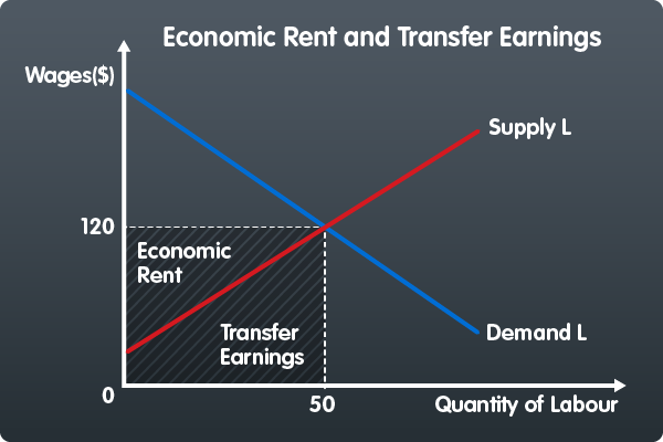
Economic Rent and Transfer Earnings To most of us “rent” is defined as a periodical payment made for the use of a particular asset – usually a residential or commercial property. However, the concept is not limited to land or buildings because it can also be applied to the other factors of production. When a factor is earning more than its supply price, it is receiving a part of its income in the form of economic rent. This situation arises when demand increases and supply cannot fully respond to the increases in demand. For example, labour already employed will experience an increase in income so that they must be earning more than their supply prices.
Present Wages – Wages when initially employed = Economic Rent
The minimum payment required to prevent a person transferring to another employer or another occupation is know as transfer earnings. It is determined by what the factor could earn in its next best paid employment. Transfer earnings may be regarded as the opportunity cost of keeping an employee in their present job or it may be regarded as the employee’s supply price in their present occupation. For example, if the minimum weekly wage that would persuade someone to work as a shop attendant is $200 but he or she actually receives a wage of $250, then the transfer earnings amount is $200 and he or she is receiving $50 in the form of economic rent. Therefore, economic rent can be defined as any payment to a factor of production that is in excess of transfer earnings.
The graph below shows the demand and supply for labour. The equilibrium wage is $120 with a quantity of 50 units. Total earnings is equal to $120 x 50 units of labour = $6,000 and employees receive the same wage of $120. However, all workers except the last one taken into employment were prepared to offer their services at wages less than $120. Therefore, provided the supply of labour slopes upwards (i.e. it is less than perfectly inelastic) an increase in demand will give rise to rent payments to those factors that were already employed at the original wage of $120. The area of economic rent and transfer earnings is shown in the graph below. Only the last labour unit employed earns no economic rent because the wage of $120 is the supply price to that particular labour unit.
Inelastic and Elastic labour supply
The amount of economic rent and transfer earnings in the return to labour depends upon the elasticity of supply and the level of demand. The greater the occupational mobility of labour, the smaller the element of economic rent. If labour can do a variety of occupations then quite small changes in the wage rate will cause large movements of labour into an industry when wages rise, and out of that industry when wages fall.
Very specialised labour has an inelastic supply curve. This includes surgeons, top CEOs, scientists and jobs that require high skill levels or involve significant danger and skill, eg, deep sea divers. The relatively high rewards to this labour are due to the fact that they are in very scarce supply relative to the demands for their services. Their transfer earnings will be much less than their salary because the market values outside their own specialised professions are probably very low. A frequently quoted example of earnings that contain a large amount of economic rent are those of top sports people. Today these people can earn significant amounts of money in a short period of time. A footballer such as Christiano Ronaldo earns €326 923 per week because of his ability to attract big crowds, merchandise sales and sponsorship deals when he was at Real Madrid Football Club. His skill levels are unique and in very limited supply when considering other players. This reflects a very high marginal productivity leading to a higher wage.
Some other occupations that are held in high regard by society do not command such high salaries because of their low marginal productivity. This includes nurses, firefighters, teachers, etc. Furthermore, the supply of labour for these jobs tends to be elastic because there are many people to choose from, unlike their footballing counterparts who have unique skills.
Quasi rent
Where the supply of labour is less than perfectly elastic an increase in demand will lead to some workers receiving economic rent. This rent may be of a temporary nature, however, because the higher wage may lead to an increase in supply, which in turn, lowers the wage. Increased wages might entice other workers to undertake the necessary training. The economic rent that is earned during the period before supply can be increased is referred to as quasi rent. True economic rent refers to the remuneration of factors that are fixed in supply.
Use elearneconomics for immediate personalised feedback on economic rent and transfer earnings with tasks designed for true student-centred learning and understanding that improves students results and grades.
As we approach the external exam season it is important that you are aware of current issues to do with the New Zealand and the World Economy. Examiners always like students to relate current issues to the economic theory as it gives a good impression of being well read in the subject. Only use these indicators if it is applicable to the question. Indicators that you might want to mention are below.
New Zealand’s gross domestic product (GDP) expanded by 1.7 percent in the June 2022 quarter, above market expectations.
Coming from record low interest rates the RBNZ has recently increased the OCR by 50 basis points (0.5%). They did consider 75 basis points.
A current account deficit of $7.1 billion was recorded in the June 2022 quarter, compared with a deficit of $8.8 billion in the previous quarter (in seasonally adjusted terms)
Annual inflation remains high globally, with annual inflation within the OECD averaging 10.3 percent in August.
Global Economy – October 2022
Notice that global interest rates are on the rise as the countries tackle the current inflationary problem. Within OECD member countries, annual inflation ranged from 3% in Japan to 80.2% in Turkey. Global inflation is expected to moderate next year but likely to remain above inflation targets in many economies – RBNZ 1-3%. However with the tight monetary conditions expected to remain in place until mid 2023 GDP growth will be subdued.
Use elearneconomics for immediate personalised feedback on Monetary Policy and Interest Rates with tasks designed for true student-centred learning and understanding that improves students results and grades.
Although not in the A2 syllabus we have had some great discussions in my A2 class on Modern Monetary Theory – MMT. It has its roots in the theory of John Maynard Keynes who during the Great Depression created the field of macroeconomics. He stated that the fact that income must always move to the level where the flows of saving and investment are equal leads to one of the most important paradoxes in economics – the paradox of thrift. Keynes explains how, under certain circumstances, an attempt to increase savings may lead to a fall in total savings. Any attempt to save more which is not matched by an equal willingness to invest more will create a deficiency in demand – leakages (savings) will exceed injections (investment) and income will fall to a new equilibrium. When you get this situation it is the government that can get the economy moving again by putting money in people’s pockets.
MMT states that a government that can create its own money therefore:
1. Cannot default on debt denominated in its own currency; 2. Can pay for goods, services, and financial assets without a need to collect money in the form of taxes or debt issuance in advance of such purchases; 3. Is limited in its money creation and purchases by inflation, which accelerates once the economic resources (i.e., labor and capital) of the economy are utilised at full employment; 4. Can control inflation by taxation and bond issuance, which remove excess money from circulation, although the political will to do so may not always exist; 5. Does not need to compete with the private sector for scarce savings by issuing bonds.
Within this model the only constraint on spending is inflation, which can break out if the public and private sectors spend too much at the same time. As long as there are enough workers and equipment to meet growing demand without igniting inflation, the government can spend what it needs to maintain employment and achieve goals such as halting climate change.
How does it differ from more mainstream monetary policy – see table below.
Those against MMT are dubious of the idea that the treasury and central bank should work together and also concerned about the jobs guarantee. They argue that if the government’s wage for guaranteed jobs is too low it won’t do much to help unemployed workers or the economy, while if it’s too high it will undermine private employment. They also say that trying to use fiscal policy to steer the economy is a proven failure because politicians rarely act quickly enough to respond to a downturn. They can’t be relied upon to impose pain on the public through higher taxes or lower spending to quell rising inflation.
Below is a video from Stephanie Kelton, an MMTer who was the economic adviser on Vermont Independent Senator Bernie Sanders’s presidential campaign in 2016.
Below is an interesting graphic from the FT which shows GDP and Inflation over the last couple of years in New Zealand – you can select other countries as well and it is good to compare different parts of the world. Note that NZ’s inflation and GDP is lower than the global average. You would normally experience stagflation when the stagnant growth is accompanied by high levels of unemployment – NZ has 3.3% unemployment. However the labour markets globally are very tight with just today British Airways cancelling 10,000 flights due to labour shortages.
If you look at Japan you will see very little difference between GDP and Inflation and you could say they may be eventually coming out of a deflationary period.
Michael Cameron in his blog ‘Sex, Drugs and Economics’ wrote a piece on full employment and the fact that it doesn’t benefit all workers. It was based on his published article in The Conversation.
Full employment has normally been the concept that has been used to describe a situation where there is no cyclical or deficient-demand unemployment, but unemployment does exist as allowances must be made for frictional unemployment and seasonal factors – also referred to as the natural rate of unemployment or Non-Accelerating Inflation Rate of Unemployment (NAIRU). Full employment does suggest that the employee has a lot of bargaining power as the supply of labour is scarce relative to the demand. In theory a tight labour market should lead to higher wages and improved conditions of work as the employer has less labour to chose from. We have seen in the labour market incentives for employees in recommending potential candidates for vacancies in the company. Other incentives for potential employees include shorter working weeks, hiring bonuses and special leave days.
However this doesn’t apply to all workers as Michael Cameron alludes to. A lot depends on the bargaining power of the worker and the elasticity of supply of labour. If the supply is very inelastic for a particular job (higher skilled) it is harder and most likely more expensive for the employer to find an alternative worker. This is evident when unemployment is low as the worker can easily look around at other job opportunities. On the contrary if the supply of labour is more elastic (lower skilled jobs) the worker has less bargaining power and the employer will have more potential workers to chose from. The graph below shows the elasticity of supply of labour – high skilled has a steeper curve (inelastic) whilst low skilled as a flatter curve (elastic)
Many low-income workers are in jobs that are part-time, fixed-term or precarious. Low-wage workers are not benefiting from the tight labour market to the same extent as more highly qualified workers.
Nevertheless, a period of full employment may allow some low-wage workers to move into higher paying jobs, or jobs that are less precarious and/or offer better work conditions. That relies on the workers having the appropriate skills and experience for higher-paying jobs, or for increasingly desperate employers to adjust their employment standards to meet those of the available job applicants.
Add to this the increase in the cost of living and those in low skilled jobs with little bargaining power are under pressure to accept whatever is available. The alternative is welfare benefits which are always playing catch-up
Below are figures and a graph for the NZ labour market from 2020 – 2022. Although the unemployed figures have fallen to 3.2% of the working population, the drop in those actively looking for work – participation rate – have fallen by a similar amount. The number of those employed increased although matched by the change in the working age population. This gives the impression that people who were previously unemployed in 2020 have not got a job, but are not making themselves available for work. Notice the difference in the graph between the growth in employment and the unemployment rate from 2020 onwards. Also the majority of extra jobs in the economy have been full-time roles as employers struggled to find labour.
Below is a flow chart that shows how you calculate the participation rate, unemployment rate etc with some older figures. This is important for MCQ as well as essays on the labour market.
Sign up to elearneconomics for multiple choice test questions (many with coloured diagrams and models) and the reasoned answers on Unemployment. Immediate feedback and tracked results allow students to identify areas of strength and weakness vital for student-centred learning and understanding.
There are those that see the problem of unemployment in most economies (but especially the US) as a structural issue. This refers to the mismatch between the jobs that are available and the skills that people have. Cyclical unemployment can be reduced by boosting demand – dropping taxes and increasing government spending (fiscal policy) and lowering interest rates (monetary policy). However, if unemployment is mainly structural patience is needed to wait for the market to sort things out, and this takes time.
The Beveridge curve is an empirical relationship between job openings (vacancies) and unemployment. It serves as a simple representation of how efficient labour markets are in terms of matching unemployed workers to available job openings in the aggregate economy. Economists study movements in this curve to identify changes in the efficiency of the labour market. It is common to observe movements along this curve over the course of the business cycle. For instance, as the economy moves into a recession, unemployment goes up and firms post fewer vacancies, causing the equilibrium in the labor market to move downward along the curve (the red arrows in the figure above). Conversely, as the economy expands, firms look for new hires to increase their production and meet demand, which depletes the stock of the unemployed – see graph below.
Careful analysis of Beveridge Curve data by economists Murat Tasci and John Lindner at the Cleveland Federal Reserve shows that it’s behaving much the way it has in previous recessions: there are as few job vacancies as you’d expect, given how desperate people are for work – see graph below. The percentage of small businesses with so-called “hard-to-fill” job vacancies is near a twenty-five-year low, and open jobs are being filled quickly. And one recent study showed that companies’ “recruiting intensity” has dropped sharply, probably because the fall-off in demand means that they don’t have a pressing need for new workers.
The Beveridge Curve and COVID
The graph below shows the Beveridge Curve pre and post covid. The pre-covid curve is a typical which relates to theory above, however the post-covid curve has become a lot steeper in showing that changes in the unemployment rate are not as responsive to changes in the vacancies. If the matching process between workers and firms becomes less efficient, employers need to post more vacancies to fill a given number of positions. In terms of the model, an outward shift of the Beveridge curve can therefore be explained by a decline in match efficiency. Since match efficiency has declined, any reduction in unemployment now requires a much higher job opening rate than before the pandemic. During the pandemic, job creation has become more difficult, and firms have had to recruit more aggressively to find workers. Looking forward, a reduction of the unemployment rate to pre-COVID levels would require job openings to be at twice the level they were before.
Source: Revisiting the Beveridge Curve: Why has it shifter so dramatically. Economic Brief October 2021
The Inflation globally has been on the increase and above the target band in most developed economies. This applies to both Headline and Core inflation.
Headline Inflation – all goods and services Core Inflation – all goods and services excluding food and energy.
Economic theory suggests that inflation could accelerate and return to levels seen in the 1970’s. A lot will depend how policymakers react to the challenge of bringing inflation down to their specific target level – RBNZ 1-3% but CPI in NZ is 5.9%. See chart for inflation breakdown in OECD countries.
Source: IMF
Key reasons for inflationary pressure.
Supply chain bottlenecks: Lockdowns and shipping problems (container shortages) but latterly the demand side has accelerated – economic recovery and demand for durable goods as well as panic buying.
Demand for more goods than services: Much of the inflation has been in durable goods whilst service inflation has only seen a small increase. This is dependent on which country – for instance demand for used cars in the US has soared.
Fiscal and Monetary stimulus: Approximately US$16.9trn of government spending has been injected into the global economy. This is accompanied by expansionary monetary policy (low interest rates) is conducive to more spending and higher inflation. Savings that accumulated during the lockdowns were now being spent. There was a debate between leading economists whether the inflation would be transitory or persistent. It seems that the data now supports those of the persistent camp. Whether it persists depends on central banks.
Labour supply: Labour participation rates have dropped – for instance for every job opening in the US there is only 0.77 unemployed people per job. See previous post – US Economy – potential for wage-price spiral. This is due to continue meaning that there is a job seekers market where there is likely to be pressure on wages.
Russian invasion of Ukraine: Russia and Ukraine are big exporters of food and major commodities so higher prices have been inevitable with major disruptions to the supply either through sanctions or conflict areas. They supply 30% of global wheat exports so prices have been increasing.
Source: IMF
What should central banks do?
Mainstream policy by central bankers should ignore supply-side shocks like higher commodity prices as this is only temporary. When central banks have intervened and raised interest rates they have ended up worsening economic conditions – ECB raising rates post GFC in 2008 and 2011. Already inflation globally is increasing but there is little central banks can do with higher global energy prices. A focus on home grown inflation (core) might be a better indicator to watch as well as the labour market – fast wage growth might mean higher interest rates. Economist John Cochrane argues that bringing down inflation through higher interest rate is a blunt tool, especially when prices have risen predominately through a loose fiscal policy. He states that inflation might get worse if people doubt the government’s ability to repay its debt without a discount from inflation.
Ultimately the outlook for inflation depends on how determined central banks are to rein in inflation and the confidence of the bond market to governments willingness to pay their debts. Below is a good video from the IMF on the inflationary problem.